Return Forecasting: Time Series Analysis & Modelling with CAD-PHY Exchange rate data.

In this notebook, you will load historical Canadian Dollar-Yen exchange rate futures data and apply time series analysis and modeling to determine whether there is any predictable behavior.

import numpy as np
import pandas as pd
from pathlib import Path
%matplotlib inline

import warnings
warnings.simplefilter(action='ignore', category=Warning)

# Currency pair exchange rates for CAD/JPY
cad_jpy_df = pd.read_csv(
    Path("cad_jpy.csv"), index_col="Date", infer_datetime_format=True, parse_dates=True
)
cad_jpy_df.head()

	Price	Open	High	Low
Date
1982-01-05	184.65	184.65	184.65	184.65
1982-01-06	185.06	185.06	185.06	185.06
1982-01-07	186.88	186.88	186.88	186.88
1982-01-08	186.58	186.58	186.58	186.58
1982-01-11	187.64	187.64	187.64	187.64

# Trim the dataset to begin on January 1st, 1990
cad_jpy_df = cad_jpy_df.loc["1990-01-01":, :]
cad_jpy_df.head()

	Price	Open	High	Low
Date
1990-01-02	126.37	126.31	126.37	126.31
1990-01-03	125.30	125.24	125.30	125.24
1990-01-04	123.46	123.41	123.46	123.41
1990-01-05	124.54	124.48	124.54	124.48
1990-01-08	124.27	124.21	124.27	124.21

Initial Time-Series Plotting

Start by plotting the “Settle” price. Do you see any patterns, long-term and/or short?

# Plot just the "Price" column from the dataframe:
cad_jpy_df[["Price"]].plot(figsize=(15,10), title="CAD/JPY Exchange Rates")

<AxesSubplot:title={'center':'CAD/JPY Exchange Rates'}, xlabel='Date'>

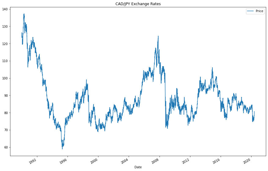
Question: Do you see any patterns, long-term and/or short?

Answer:

Let us review the trends in the 1990s first. There is a significant drop in the price, but by the end of the 1990s there was a marginal resurgance. From 2000 until approximately 2008, we can see a significant upwards trend, with many smaller peaks and valleys. In the short term, therefore, we can see volatility abound. In the long term, we see a sharp decline and a long-standing resurgence of the price. Around the present year, we see almost the same pricing as in the 1990s.

Decomposition Using a Hodrick-Prescott Filter

Using a Hodrick-Prescott Filter, decompose the exchange rate price into trend and noise.

import statsmodels.api as sm

# Apply the Hodrick-Prescott Filter by decomposing the exchange rate price into two separate series:
ts_noise, ts_trend = sm.tsa.filters.hpfilter(cad_jpy_df['Price'])

# Plot the trend
ts_trend.plot()

<AxesSubplot:xlabel='Date'>

# Create a dataframe of just the exchange rate price, and add columns for "noise" and "trend" series from above:
combined_df = cad_jpy_df[["Price"]]
combined_df['noise'] = ts_noise
combined_df['trend'] = ts_trend
combined_df.head()

	Price	noise	trend
Date
1990-01-02	126.37	0.519095	125.850905
1990-01-03	125.30	-0.379684	125.679684
1990-01-04	123.46	-2.048788	125.508788
1990-01-05	124.54	-0.798304	125.338304
1990-01-08	124.27	-0.897037	125.167037

 combined_df[["Price", "trend"]]["2015-01-01":"2020-06-04"].plot(figsize=(15,10), title="Price vs. Trend")

<AxesSubplot:title={'center':'Price vs. Trend'}, xlabel='Date'>

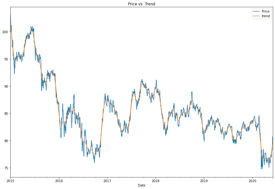
Question: Do you see any patterns, long-term and/or short?

Answer:

Let us review the trends after applying the HP Filter. First, as may be predicted, the HP filter will smooth out the peaks and valleys. That is predicted because the purpose of the HP filter is to remove the fluctuations that do not add salience or relevance to our analysis. In the short term, we again see annual dips and peaks that correspond slightly with the months of the year- especially in 2018 and 2019. In the long term, we see a significant decline with a slight increase. The price has not yet regained its 2015 value as of the 2020 price indicators. Thus we can conclude an overall decline.

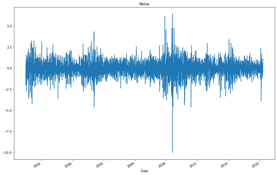
# Plot the settle noise
ts_noise.plot(figsize=(15,10), title="Noise")

<AxesSubplot:title={'center':'Noise'}, xlabel='Date'>

---

Forecasting Returns using an ARMA Model

Using exchange rate Returns, estimate an ARMA model

1. ARMA: Create an ARMA model and fit it to the returns data. Note: Set the AR and MA (“p” and “q”) parameters to p=2 and q=1: order=(2, 1).
2. Output the ARMA summary table and take note of the p-values of the lags. Based on the p-values, is the model a good fit (p < 0.05)?
3. Plot the 5-day forecast of the forecasted returns (the results forecast from ARMA model)

# Create a series using "Price" percentage returns, drop any nan"s, and check the results:
# (Make sure to multiply the pct_change() results by 100)
# In this case, you may have to replace inf, -inf values with np.nan"s
returns = (cad_jpy_df[["Price"]].pct_change() * 100)
returns = returns.replace(-np.inf, np.nan).dropna()
returns.tail()

	Price
Date
2020-05-29	0.076697
2020-06-01	1.251756
2020-06-02	1.425508
2020-06-03	0.373134
2020-06-04	0.012392

returns.head()

	Price
Date
1990-01-03	-0.846720
1990-01-04	-1.468476
1990-01-05	0.874777
1990-01-08	-0.216798
1990-01-09	0.667901

# Import the ARMA model
import statsmodels.api as sm
from scipy import stats
from statsmodels.tsa.arima.model import ARIMA

# use order=(2, 1).

# Estimate and ARMA model using statsmodels (use order=(2, 1))
model = ARIMA(returns.values, order=(2, 1,0))

# Fit the model and assign it to a variable called results
results = model.fit()

print(results.params)

[-0.68605843 -0.33420741  0.92386488]

# Output model summary results:
results.summary()

SARIMAX Results

Dep. Variable:	y	No. Observations:	7928
Model:	ARIMA(2, 1, 0)	Log Likelihood	-10934.368
Date:	Fri, 11 Feb 2022	AIC	21874.736
Time:	14:20:12	BIC	21895.670
Sample:	0	HQIC	21881.904
	- 7928
Covariance Type:	opg

	coef	std err	z	P>|z|	[0.025	0.975]
ar.L1	-0.6861	0.006	-110.065	0.000	-0.698	-0.674
ar.L2	-0.3342	0.006	-51.510	0.000	-0.347	-0.321
sigma2	0.9239	0.008	121.627	0.000	0.909	0.939

Ljung-Box (L1) (Q):	59.79	Jarque-Bera (JB):	11829.47
Prob(Q):	0.00	Prob(JB):	0.00
Heteroskedasticity (H):	0.83	Skew:	0.27
Prob(H) (two-sided):	0.00	Kurtosis:	8.96

Warnings:
[1] Covariance matrix calculated using the outer product of gradients (complex-step).

print(results.forecast(steps=5)[:])

[0.61159318 0.32106877 0.32012787 0.4178688  0.35112727]

# Plot the 5 Day Returns Forecast
pd.DataFrame(results.forecast(steps=5)[:]).plot(title="5 Day Returns Forecast")

<AxesSubplot:title={'center':'5 Day Returns Forecast'}>

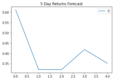
Question: Based on the p-value, is the model a good fit?

Answer:

Since our p-value >α, we can determine that the model is not a good fit. Specifically, in this case, 2 > 0.5, thus p-value >α.

---

Forecasting the Exchange Rate Price using an ARIMA Model

1. Using the raw CAD/JPY exchange rate price, estimate an ARIMA model.
   1. Set P=5, D=1, and Q=1 in the model (e.g., ARIMA(df, order=(5,1,1))
   2. P= # of Auto-Regressive Lags, D= # of Differences (this is usually =1), Q= # of Moving Average Lags
2. Output the ARIMA summary table and take note of the p-values of the lags. Based on the p-values, is the model a good fit (p < 0.05)?
3. Plot a 5 day forecast for the Exchange Rate Price. What does the model forecast predict will happen to the Japanese Yen in the near term?

# Currency pair exchange rates for CAD/JPY
cad_jpy_new_df = pd.read_csv(
    Path("cad_jpy.csv"), index_col="Date", infer_datetime_format=True, parse_dates=True
)
cad_jpy_new_df.head()

	Price	Open	High	Low
Date
1982-01-05	184.65	184.65	184.65	184.65
1982-01-06	185.06	185.06	185.06	185.06
1982-01-07	186.88	186.88	186.88	186.88
1982-01-08	186.58	186.58	186.58	186.58
1982-01-11	187.64	187.64	187.64	187.64

returns2 = (cad_jpy_new_df[["Price"]].pct_change())
returns2 = returns.replace(-np.inf, np.nan).dropna()
returns2.tail()

	Price
Date
2020-05-29	0.076697
2020-06-01	1.251756
2020-06-02	1.425508
2020-06-03	0.373134
2020-06-04	0.012392

 y = cad_jpy_df["Price"].to_frame()

 y.dtypes

Price    float64
dtype: object

from statsmodels.tsa.arima.model import ARIMA

#utilize order=(5,1,1))

# Estimate and ARIMA Model:
# Hint: ARIMA(df, order=(p, d, q))

model = ARIMA( y, order=(5, 1, 1))

# Fit the model
results2 = model.fit()

C:\Users\benja\anaconda3\lib\site-packages\statsmodels\tsa\base\tsa_model.py:593: ValueWarning: A date index has been provided, but it has no associated frequency information and so will be ignored when e.g. forecasting.
  warnings.warn('A date index has been provided, but it has no'
C:\Users\benja\anaconda3\lib\site-packages\statsmodels\tsa\base\tsa_model.py:593: ValueWarning: A date index has been provided, but it has no associated frequency information and so will be ignored when e.g. forecasting.
  warnings.warn('A date index has been provided, but it has no'
C:\Users\benja\anaconda3\lib\site-packages\statsmodels\tsa\base\tsa_model.py:593: ValueWarning: A date index has been provided, but it has no associated frequency information and so will be ignored when e.g. forecasting.
  warnings.warn('A date index has been provided, but it has no'

print(results2.params)

ar.L1     0.430330
ar.L2     0.017827
ar.L3    -0.011751
ar.L4     0.010993
ar.L5    -0.019068
ma.L1    -0.458295
sigma2    0.531769
dtype: float64

# Output model summary results:
results2.summary()

SARIMAX Results

Dep. Variable:	Price	No. Observations:	7929
Model:	ARIMA(5, 1, 1)	Log Likelihood	-8745.898
Date:	Fri, 11 Feb 2022	AIC	17505.796
Time:	14:20:16	BIC	17554.643
Sample:	0	HQIC	17522.523
	- 7929
Covariance Type:	opg

	coef	std err	z	P>|z|	[0.025	0.975]
ar.L1	0.4303	0.331	1.299	0.194	-0.219	1.080
ar.L2	0.0178	0.012	1.459	0.145	-0.006	0.042
ar.L3	-0.0118	0.009	-1.313	0.189	-0.029	0.006
ar.L4	0.0110	0.008	1.299	0.194	-0.006	0.028
ar.L5	-0.0191	0.007	-2.706	0.007	-0.033	-0.005
ma.L1	-0.4583	0.332	-1.381	0.167	-1.109	0.192
sigma2	0.5318	0.004	118.418	0.000	0.523	0.541

Ljung-Box (L1) (Q):	0.00	Jarque-Bera (JB):	9233.72
Prob(Q):	0.97	Prob(JB):	0.00
Heteroskedasticity (H):	0.78	Skew:	-0.58
Prob(H) (two-sided):	0.00	Kurtosis:	8.16

Warnings:
[1] Covariance matrix calculated using the outer product of gradients (complex-step).

# Plot the 5 Day Price Forecast
pd.DataFrame(results2.forecast(steps=5)[:]).plot(title="5 Day Futures Price Forecast")

C:\Users\benja\anaconda3\lib\site-packages\statsmodels\tsa\base\tsa_model.py:390: ValueWarning: No supported index is available. Prediction results will be given with an integer index beginning at `start`.
  warnings.warn('No supported index is available.'





<AxesSubplot:title={'center':'5 Day Futures Price Forecast'}>

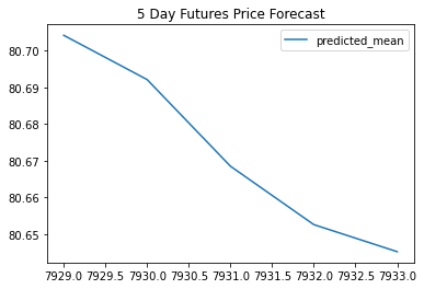
Question: What does the model forecast will happen to the Japanese Yen in the near term?

Answer:

My model forecases that the Japanese Yen will weaken in the near term. The plot titled “5 Day Futures Price Forecast” clearly shows a steep decline.

---

Volatility Forecasting with GARCH

Rather than predicting returns, let’s forecast near-term volatility of Japanese Yen exchange rate returns. Being able to accurately predict volatility will be extremely useful if we want to trade in derivatives or quantify our maximum loss.

Using exchange rate Returns, estimate a GARCH model. Hint: You can reuse the returns variable from the ARMA model section.

1. GARCH: Create an GARCH model and fit it to the returns data. Note: Set the parameters to p=2 and q=1: order=(2, 1).
2. Output the GARCH summary table and take note of the p-values of the lags. Based on the p-values, is the model a good fit (p < 0.05)?
3. Plot the 5-day forecast of the volatility.

import arch as arch
from arch import arch_model

returns = (cad_jpy_df[["Price"]].pct_change() * 100)
returns = returns.replace(-np.inf, np.nan).dropna()
returns.head()

	Price
Date
1990-01-03	-0.846720
1990-01-04	-1.468476
1990-01-05	0.874777
1990-01-08	-0.216798
1990-01-09	0.667901

# Estimate a GARCH model:
model = arch_model(returns, mean="Zero", vol="GARCH", p=2, q=1)

# Fit the model
res = model.fit(disp="off")

# Summarize the model results
res.summary()

Zero Mean - GARCH Model Results

Dep. Variable:	Price	R-squared:	0.000
Mean Model:	Zero Mean	Adj. R-squared:	0.000
Vol Model:	GARCH	Log-Likelihood:	-8911.02
Distribution:	Normal	AIC:	17830.0
Method:	Maximum Likelihood	BIC:	17858.0
		No. Observations:	7928
Date:	Fri, Feb 11 2022	Df Residuals:	7928
Time:	14:20:17	Df Model:	0

Volatility Model

	coef	std err	t	P>|t|	95.0% Conf. Int.
omega	9.0733e-03	2.545e-03	3.566	3.628e-04	[4.086e-03,1.406e-02]
alpha[1]	0.0624	1.835e-02	3.402	6.682e-04	[2.647e-02,9.841e-02]
alpha[2]	0.0000	2.010e-02	0.000	1.000	[-3.940e-02,3.940e-02]
beta[1]	0.9243	1.229e-02	75.205	0.000	[ 0.900, 0.948]

Covariance estimator: robust

Note: Our p-values for GARCH and volatility forecasts tend to be much lower than our ARMA/ARIMA return and price forecasts. In particular, here we have all p-values of less than 0.05, except for alpha(2), indicating overall a much better model performance. In practice, in financial markets, it’s easier to forecast volatility than it is to forecast returns or prices. (After all, if we could very easily predict returns, we’d all be rich!)

# Find the last day of the dataset
last_day = returns.index.max().strftime('%Y-%m-%d')
last_day

'2020-06-04'

# Create a 5 day forecast of volatility
forecast_horizon = 5

# Start the forecast using the last_day calculated above
forecasts = res.forecast(start='2020-06-04', horizon=forecast_horizon, reindex=False)
forecasts

<arch.univariate.base.ARCHModelForecast at 0x1f995aa9bb0>

# Annualize the forecast
intermediate = np.sqrt(forecasts.variance.dropna() * 252)
intermediate.head()

	h.1	h.2	h.3	h.4	h.5
Date
2020-06-04	12.566029	12.573718	12.581301	12.588778	12.596153

# Transpose the forecast so that it is easier to plot
final = intermediate.dropna().T
final.head()

Date	2020-06-04
h.1	12.566029
h.2	12.573718
h.3	12.581301
h.4	12.588778
h.5	12.596153

# Plot the final forecast
final.plot(title="5 Day Forecast of Volatility")

<AxesSubplot:title={'center':'5 Day Forecast of Volatility'}>

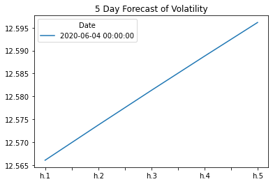
Question: What does the model forecast will happen to volatility in the near term?

Answer:

The model indicates that the volatility will increase in the near term. The five day forecast clearly shows the increase from h1 to h5.

---

Conclusions

Based on your time series analysis, would you buy the yen now?

Answer:

The volatility of the Yen indicated by the GARCH model indicates that purchasing the yen now would not be a wise investment option.

Is the risk of the yen expected to increase or decrease?

Answer:

The volatility of the Yen predicts that the risk associated with the Yen is on the rise. However, it should be noted that this only a short term conclusion. In the future the risk may vary upwards or downwards depending on a variety of factors.

Based on the model evaluation, would you feel confident in using these models for trading?

Answer:

The fit of a model should be determined by p-value >α. These models have shown that they are not a good fit, and would therefore require further modifications and calibrations to be fit for trading purposes. They could be tweaked, and over time may be suitable. But at the present time these p-values indicate that the models are not a good fit- and therefore not suitable for trading purposes.