Regression Analysis: Currency Analysis with Sklearn Linear Regression

In this notebook, you will build a SKLearn linear regression model to predict Yen futures (“settle”) returns with lagged CAD/JPY exchange rate returns.

import numpy as np
import pandas as pd
from pathlib import Path
%matplotlib inline

# Currency pair exchange rates for CAD/JPY
cad_jpy_df = pd.read_csv(
    Path("cad_jpy.csv"), index_col="Date", infer_datetime_format=True, parse_dates=True
)
cad_jpy_df.head()

	Price	Open	High	Low
Date
1982-01-05	184.65	184.65	184.65	184.65
1982-01-06	185.06	185.06	185.06	185.06
1982-01-07	186.88	186.88	186.88	186.88
1982-01-08	186.58	186.58	186.58	186.58
1982-01-11	187.64	187.64	187.64	187.64

# Trim the dataset to begin on January 1st, 1990
cad_jpy_df = cad_jpy_df.loc["1990-01-01":, :]
cad_jpy_df.head()

	Price	Open	High	Low
Date
1990-01-02	126.37	126.31	126.37	126.31
1990-01-03	125.30	125.24	125.30	125.24
1990-01-04	123.46	123.41	123.46	123.41
1990-01-05	124.54	124.48	124.54	124.48
1990-01-08	124.27	124.21	124.27	124.21

Data Preparation

Returns

# Create a series using "Price" percentage returns, drop any nan"s, and check the results:
# (Make sure to multiply the pct_change() results by 100)
# In this case, you may have to replace inf, -inf values with np.nan"s
cad_jpy_df["Return"] = cad_jpy_df[["Price"]].pct_change() * 100
cad_jpy_df = cad_jpy_df.replace(-np.inf, np.nan).dropna()
cad_jpy_df.tail()

	Price	Open	High	Low	Return
Date
2020-05-29	78.29	78.21	78.41	77.75	0.076697
2020-06-01	79.27	78.21	79.36	78.04	1.251756
2020-06-02	80.40	79.26	80.56	79.15	1.425508
2020-06-03	80.70	80.40	80.82	79.96	0.373134
2020-06-04	80.71	80.80	80.89	80.51	0.012392

Lagged Returns

# Create a lagged return using the shift function
cad_jpy_df['Lagged_Return'] = cad_jpy_df.Return.shift()
cad_jpy_df =cad_jpy_df.dropna()
cad_jpy_df.tail()

	Price	Open	High	Low	Return	Lagged_Return
Date
2020-05-29	78.29	78.21	78.41	77.75	0.076697	-0.114913
2020-06-01	79.27	78.21	79.36	78.04	1.251756	0.076697
2020-06-02	80.40	79.26	80.56	79.15	1.425508	1.251756
2020-06-03	80.70	80.40	80.82	79.96	0.373134	1.425508
2020-06-04	80.71	80.80	80.89	80.51	0.012392	0.373134

Train Test Split

# Create a train/test split for the data using 2018-2019 for testing and the rest for training
train = cad_jpy_df[:'2017']
test = cad_jpy_df['2018':]

# Create four dataframes:
# X_train (training set using just the independent variables), X_test (test set of of just the independent variables)
# Y_train (training set using just the "y" variable, i.e., "Futures Return"), Y_test (test set of just the "y" variable):
X_train = train["Lagged_Return"].to_frame()
X_test = test["Lagged_Return"].to_frame()
y_train = train["Return"]
y_test = test["Return"]

# Preview the X_train data
X_train.head()

	Lagged_Return
Date
1990-01-04	-0.846720
1990-01-05	-1.468476
1990-01-08	0.874777
1990-01-09	-0.216798
1990-01-10	0.667901

Linear Regression Model

# Create a Linear Regression model and fit it to the training data
from sklearn.linear_model import LinearRegression

# Fit a SKLearn linear regression using  just the training set (X_train, Y_train):
model = LinearRegression()
model.fit(X_train, y_train)

LinearRegression()

Make predictions using the Testing Data

Note: We want to evaluate the model using data that it has never seen before, in this case: X_test.

# Make a prediction of "y" values using just the test dataset
predictions = model.predict(X_test)

# Assemble actual y data (Y_test) with predicted y data (from just above) into two columns in a dataframe:
Results = y_test.to_frame()
Results["Predicted Return"] = predictions
Results.head(5)

	Return	Predicted Return
Date
2018-01-01	0.245591	0.005434
2018-01-02	-0.055679	-0.007317
2018-01-03	0.011142	0.000340
2018-01-04	0.601604	-0.001358
2018-01-05	0.919158	-0.016366

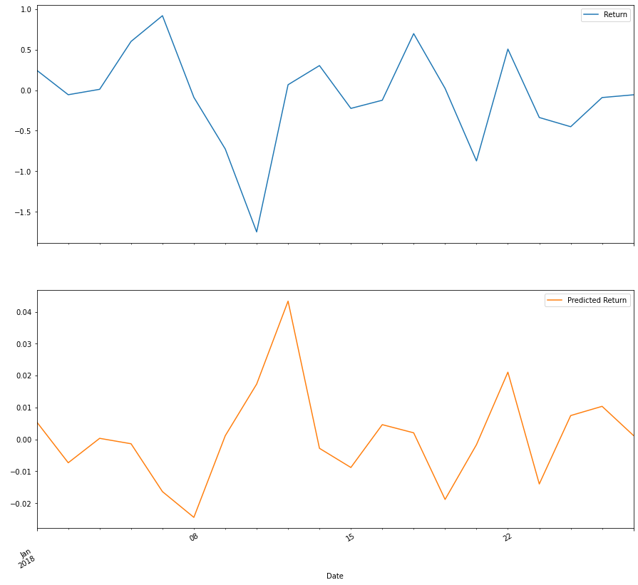
# Plot the first 20 predictions vs the true values

# The trends lines should be similar
Results[:20].plot(subplots=True, figsize=(15,15))

array([<AxesSubplot:xlabel='Date'>, <AxesSubplot:xlabel='Date'>],
      dtype=object)

Out-of-Sample Performance

Evaluate the model using “out-of-sample” data (X_test and y_test)

from sklearn.metrics import mean_squared_error
# Calculate the mean_squared_error (MSE) on actual versus predicted test "y" 
# (Hint: use the dataframe from above)
mse = mean_squared_error(
    Results["Return"],
    Results["Predicted Return"]
)

# Using that mean-squared-error, calculate the root-mean-squared error (RMSE):
rmse = np.sqrt(mse)
print(f"Out-of-Sample Root Mean Squared Error (RMSE): {rmse}")

Out-of-Sample Root Mean Squared Error (RMSE): 0.6445805658569028

In-Sample Performance

Evaluate the model using in-sample data (X_train and y_train)

# Construct a dataframe using just the "y" training data:
in_sample_results = y_train.to_frame()

# Add a column of "in-sample" predictions to that dataframe:  
in_sample_results["In-sample Predictions"] = model.predict(X_train)

# Calculate in-sample mean_squared_error (for comparison to out-of-sample)
in_sample_mse = mean_squared_error(
    in_sample_results["Return"],
    in_sample_results["In-sample Predictions"]
)

# Calculate in-sample root mean_squared_error (for comparison to out-of-sample)
in_sample_rmse = np.sqrt(in_sample_mse)
print(f"In-sample Root Mean Squared Error (RMSE): {in_sample_rmse}")

In-sample Root Mean Squared Error (RMSE): 0.841994632894117

Conclusions

Question: Does this model perform better or worse on out-of-sample data as compared to in-sample data?

Answer: With a lower RMSE, we have a better model. So with that in mind, we can conclude that the out-of-sample performance is better than our in-sample performance. The In-Sample performance RMSE is close to 1, whereas the RMSE for the out-of-sample is closer to 0.5. Thus, this model performs better on the out-of-sample performance.